Tuning Kafka for Sub Second Pipelines

Before you even think about touching a configuration file, let's be clear: tuning Kafka for sub-second performance is a science, not a guessing game. It all starts with defining exactly what you're trying to achieve and setting up a solid way to measure your progress. You need to move beyond vague goals like "make it faster" and set concrete Service Level Objectives (SLOs), like aiming for a 99th percentile (p99) latency under 500 milliseconds.

Defining Your Sub-Second Performance Goals

The first question I always ask is, what does "fast" really mean for your application? The sub-second target for a real-time fraud detection system is worlds apart from what's needed for a simple log aggregation pipeline. Getting this definition right from the start ensures your tuning efforts are laser-focused on what actually matters to the business.

Your first practical step is to build a benchmarking environment that’s a dead ringer for production. I can't stress this enough—using production-like hardware, network conditions, and data patterns is non-negotiable. If you skimp here, your tests will be misleading, and you'll end up optimizing for the wrong things.

Key Metrics to Monitor

To truly understand your pipeline's health, you have to look beyond simple averages. Averages lie; they can easily hide the painful latency outliers that are frustrating your users. Instead, zero in on the metrics that tell the real story.

• p95/p99 Latency: This is your window into the "worst-case" experience for the vast majority of your messages. If you can keep your p99 latency low, you know your pipeline is consistently fast, not just fast on average.
• End-to-End Latency: This is the ultimate source of truth. It measures the total time a message takes from the producer sending it to the consumer finishing its processing.
• Throughput: You need to know how much data you can push, usually measured in messages per second or MB/s. Be careful here, as aggressive latency tuning can sometimes tank your throughput.
• Consumer Lag: This tells you how far behind your consumers are from the newest message. If lag is piling up, it's a dead giveaway that your consumers can't keep up.

This table illustrates how different latency targets (SLOs) align with specific business requirements, helping you define the right performance goals for your pipeline.

Table: Key Latency SLOs vs. Business Impact

By mapping your use case to a specific SLO, you create a clear, measurable target that guides every tuning decision you make.

Establishing a Performance Baseline

Once you have your environment and metrics locked in, it’s time to establish a baseline. Run a series of load tests using tools like the official Kafka performance scripts (kafka-producer-perf-test.sh and kafka-consumer-perf-test.sh) or something more sophisticated like JMeter or Gatling. Do this with your default Kafka configurations to see where you stand right out of the box.

By creating a reliable baseline, you transform tuning from a guessing game into a scientific process. Every configuration change can be tested and its impact—positive or negative—can be measured against this initial benchmark.

This baseline becomes your yardstick for every optimization that follows. It's also where you'll immediately confront the classic trade-offs of any distributed system. When you're chasing sub-second performance, the tug-of-war between latency and throughput is front and center. For a deeper dive into these fundamentals, our guide on real-time data streaming is a great resource. Pushing for lower latency often means sacrificing some throughput, and vice versa. This data-driven benchmarking is the only way to make informed decisions and achieve consistently fast, predictable performance.

Fine-Tuning Kafka Producers for Minimum Latency

Your quest for sub-second latency starts right at the source: the Kafka producer. This is your first, and arguably most important, chance to control how fast messages hit the wire. Simply accepting the default settings is a surefire way to get average results. If you want truly low latency, you need to get hands-on with the configuration.

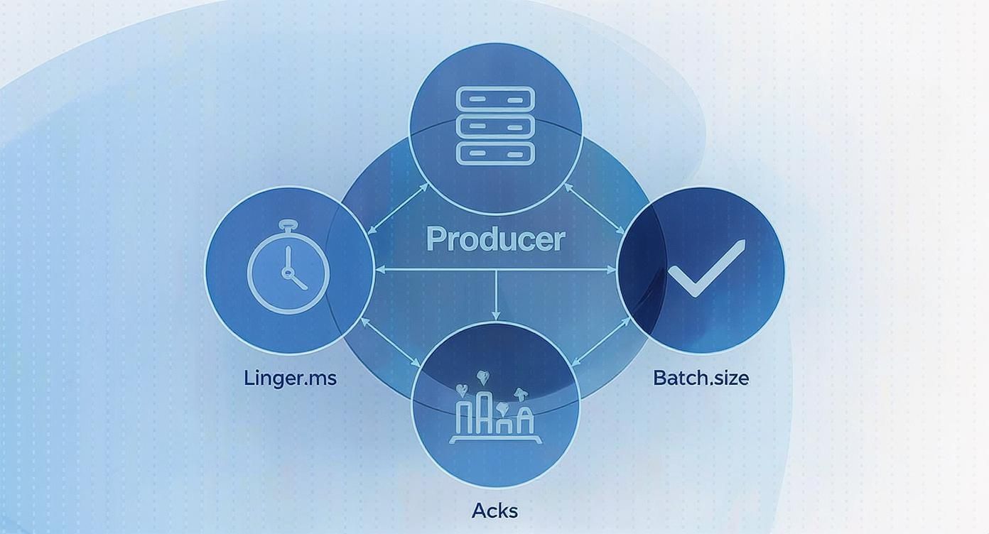
The biggest culprits for latency are almost always related to batching. Kafka producers are built for massive throughput, and they get it by bundling messages into batches before shipping them off to a broker. While fantastic for efficiency, this is a built-in delay. Your two main levers here are batch.size and linger.ms.

The Linger vs. Batch Size Balancing Act

Think of linger.ms as a "wait for more messages" timer. The producer will pause for this many milliseconds, hoping to collect more records to fill a batch. On the other hand, batch.size is a hard limit on how big a batch can get in bytes. The producer sends a batch as soon as either of these conditions is met.

For a sub-second pipeline, your first instinct should be to get aggressive with linger.ms.

Setting linger.ms=0 is the most direct way to attack latency. It tells the producer to send messages the moment they're ready, with no artificial delay. I’ve seen this used in financial services and real-time bidding platforms where every millisecond is critical. But this isn't a free lunch. Firing off individual messages hammers your network and brokers with more requests, which can kill your overall throughput.

For an extreme low-latency setup, kicking linger.ms down to 0 or 1 is a common first step. Just keep a close eye on your broker's CPU and network I/O, because you might just trade one bottleneck for another.

This is where batch.size provides a safety net. Even with linger.ms=0, if messages are flying in faster than the producer can send them, they’ll naturally get batched up. By setting a smaller batch.size, say 16384 bytes (16 KB), you ensure that even under a heavy load, the batches stay small and get sent out frequently.

Acknowledgments: Trading Durability for Speed

Another crucial dial is acks, which controls how durable your messages are. This setting is a textbook trade-off between latency and the guarantee that your data is safe.

• acks=0: The producer sends the message and doesn't even wait for a response. This is fire-and-forget. It's the absolute fastest you can get, but it offers zero delivery guarantees.
• acks=1: The producer waits for the leader replica to confirm it got the message. This is the most common setting and usually the right balance. It adds the latency of one network round trip but confirms the message has landed.
• acks=all: The producer waits for the leader and all of its in-sync replicas to give the thumbs-up. This is for when you absolutely cannot lose a message, but it's also the slowest option by far.

For most sub-second use cases, acks=1 is the sweet spot. You get confirmation that the message is safe on the lead broker without the hefty latency penalty of waiting for every replica to catch up.

Compression and Sending Asynchronously

Don't overlook compression. It can shrink your messages, meaning they travel across the network faster. The catch? Compression and decompression burn CPU cycles on both the producer and the consumer. Choosing the right codec is key.

For low-latency work, Snappy or LZ4 are usually the best bets. Their tiny CPU footprint is more valuable than the extra bit of compression you might get from GZIP.

Finally, make sure your application code isn't undermining your efforts. Kafka producers are asynchronous and return a Future object instantly. If your code blocks on that Future after every single send, you've just turned your producer into a synchronous, high-latency mess. Use callbacks instead to handle successes or failures without stalling the main thread.

The producer is your best opportunity to shave milliseconds off your pipeline. By aggressively tuning batching, making a conscious choice on durability, and picking the right compression, you build a solid foundation. Of course, this all assumes the data is ready to be sent. For Kafka producers, the efficiency of initial data acquisition is crucial for achieving minimum latency, and exploring various data extraction techniques can offer valuable insights.

Tuning Brokers and Topics for Peak Performance

Once you've squeezed every millisecond out of your producers, your attention has to turn to the Kafka brokers. This is where the real work happens—ingesting data, replicating it across the cluster, and serving it up to consumers. A misconfigured broker can completely undo all your hard work on the producer side, becoming the primary bottleneck in your pipeline.

Optimizing the brokers means diving into the server.properties file. This file is the command center for each broker, and just a few tweaks here can make a world of difference in I/O wait times and overall processing latency.

Sizing Your Broker Thread Pools

Two of the most critical settings you'll encounter are num.network.threads and num.io.threads. These parameters control the thread pools that manage network requests and disk I/O, respectively. Think of it like staffing checkout lanes at a grocery store—too few, and you get long lines; too many, and they're just idle, wasting resources.

• num.network.threads: This pool handles all incoming requests from producers and consumers. The default is a measly 3, which is almost always too low for any serious low-latency workload. A good starting point is to set this to roughly half the number of your broker's CPU cores.
• num.io.threads: This pool takes the requests from the network threads and does the heavy lifting of writing to disk. The default of 8 is a bit more reasonable. But if you're running on modern hardware like SSDs or NVMe drives, you can often push this higher, even matching the number of cores to really maximize your disk throughput.

A common pitfall is over-allocating these threads. It seems counterintuitive, but throwing too many threads at the problem leads to excessive context switching, which can actually increase latency. Start with a sensible baseline (like half the core count for network threads), benchmark your performance, and then adjust incrementally. The goal is to achieve parallelism without creating contention.

Before you even get to the broker, your producer-side settings lay the groundwork. Decisions around linger.ms, batch.size, and acks are the first and most direct way to attack latency.

This setup directly influences the load your brokers will have to handle, so getting it right is the essential first step.

Topic Partitions and Replication Factor

Beyond the global broker settings, how you configure your topics is just as critical for balancing parallelism and fault tolerance. The number of partitions you choose for a topic is one of the biggest architectural decisions you'll make with Kafka.

Partitions are how Kafka achieves parallelism. More partitions mean more consumers can read from a topic at the same time, which is key for high-throughput systems. But there's no free lunch; each partition adds overhead. It’s another file handle for the OS to manage, it consumes memory, and it adds complexity to leader elections when a broker fails. A good rule of thumb is to align your partition count with your expected consumer group size, leaving a little room to scale up later.

The replication factor determines how many copies of your data exist across the cluster. For any production system, a replication factor of 3 is the gold standard. This allows you to lose up to two brokers without losing a single message. Just remember that every replica adds network traffic and disk I/O, as the data has to be copied across the cluster.

To get the most out of your cluster, it's crucial to understand how settings on both the producer and broker side interact to affect latency.

Producer vs. Broker Latency Tuning Parameters

Balancing these parameters is the core challenge of Kafka performance tuning. A change on the producer often necessitates a corresponding adjustment on the broker to maintain stability.

Durability vs. Latency with min.insync.replicas

This brings us to one of the most important trade-offs, which you control with min.insync.replicas (or min.isr). This setting, used when a producer sets acks=all, dictates the minimum number of replicas that must confirm a write before the leader broker sends an acknowledgment back.

Let's say you have a topic with a replication factor of 3.

• min.insync.replicas=2: The write is considered successful once the leader and at least one other replica have the message. This configuration lets you tolerate the failure of one broker while still being able to write to the topic. It's a fantastic balance between durability and performance.
• min.insync.replicas=1: Setting this to 1 is risky. If the leader accepts a write and then crashes before that message is replicated, the data is gone for good. This configuration prioritizes availability over data consistency.

For sub-second pipelines that can't afford to lose data, the combination of a replication factor of 3 and min.insync.replicas=2 is the sweet spot. It provides strong resilience without the latency penalty of waiting for every replica to acknowledge the write.

Apache Kafka has become the industry backbone for high-throughput streaming precisely because it offers this level of granular control. In fact, some research shows that implementing smart log purging and tracking in systems that consume from Kafka can slash latency by an incredible 65-75%. If you're interested in going deeper, you can learn more about how to build a successful Kafka data pipeline. By carefully tuning these broker and topic settings, you ensure that messages flow through your entire architecture with maximum speed and rock-solid reliability.

Getting Consumers to Keep Up with the Flow

You've tuned your producers and dialed in your brokers, but all that work is for nothing if your consumers can't keep up. When messages pile up on the broker waiting to be processed, you get consumer lag—the enemy of any low-latency pipeline. If your goal is sub-second delivery, your consumers have to be just as fast as the rest of the stack.

This means you can't just stick with the default consumer settings. You need to configure them to fetch and process data as soon as it lands. The whole game is about shrinking the time between a message arriving at the broker and your application finishing its work on it. The two most important knobs for this are fetch.min.bytes and fetch.max.wait.ms.

These settings are a team. fetch.min.bytes tells the broker, "Don't bother responding until you have at least this much data for me." Meanwhile, fetch.max.wait.ms acts as a safety valve, telling the broker, "Okay, you've waited long enough, send me whatever you have."

The Fetching Balancing Act

For a sub-second pipeline, you can't afford to have the consumer wait around. You want data the instant it's available. The trick is to get that data quickly without overwhelming your brokers with constant, empty requests—a scenario often called "busy polling" that just wastes CPU and network bandwidth.

A solid starting point for low-latency setups is to get aggressive with the timers.

• Set fetch.max.wait.ms to a very low value, like 100ms or even 50ms. This prevents the broker from holding data back for too long.
• Then, set fetch.min.bytes=1. This is a powerful move. It tells the broker to send a response as soon as a single byte of data is available for the consumer.

This combination is fantastic for minimizing fetch delays, getting messages into your application almost immediately.

A Word of Caution: This aggressive fetching strategy is great for latency, but it comes at a cost. It dramatically increases the number of fetch requests your consumers make. You absolutely must monitor your broker CPU and network traffic after making this change. If they spike, you may have just moved the bottleneck from the consumer to the broker itself.

Taming Your Processing Loop

Once your consumer fetches a batch of messages, it has to actually do something with them. How you handle this is the next critical step. The max.poll.records setting dictates how many records you get back in a single poll() call.

If your processing logic is lightning-fast—say, just a simple transformation or writing to a local cache—you can probably set this to a high number like 500 to maximize throughput. But if each message requires a database lookup or an API call, a large batch can be a trap. The consumer could get stuck processing for so long that Kafka thinks it's dead, triggering a painful rebalance.

For most low-latency use cases, a smaller max.poll.records (think 50-100) paired with efficient, non-blocking processing is the safer bet. The goal is to ensure your application can finish processing one batch well before the next one is due.

• Rule of Thumb: Your total processing time for a batch of records from a poll() call needs to be significantly less than max.poll.interval.ms (which defaults to 5 minutes). If you exceed this, the broker will unceremoniously kick your consumer out of the group, assuming it has crashed.

Consumer Groups and Committing Offsets

Don't forget the fundamentals. Kafka scales by distributing topic partitions across multiple consumer instances in a consumer group. To get the most parallelism, you should aim to have as many consumers in the group as you have partitions in the topic. Any extra consumers will just sit around, idle and useless.

Offset management is all about keeping track of where you are. The default enable.auto.commit=true is easy, but it's risky. The consumer might commit an offset before your application has successfully processed the corresponding message. If it crashes right after, that message is lost forever.

For any serious pipeline, you should set enable.auto.commit=false and handle commits yourself. By committing the offset only after your processing is complete, you guarantee "at-least-once" delivery, which is crucial for data integrity.

Finally, take a look at your partition assignment strategy. The default, RangeAssignor, can sometimes bunch partitions onto a few consumers during a rebalance. Consider switching to the StickyAssignor. Its goal is to minimize partition movement when consumers join or leave the group. This means rebalances are less disruptive and your system gets back to its high-performance rhythm much faster.

Advanced Tuning: Hardware, OS, and JVM

If you're serious about pushing Kafka into sub-second territory, you eventually have to look past its configuration files and start tuning the very foundation it runs on. Elite performance is a full-stack effort. When every millisecond counts, your hardware, operating system, and the Java Virtual Machine (JVM) itself become critical levers you can pull.

Even the most carefully tuned producer and broker settings can be completely kneecapped by a sluggish disk or a poorly configured JVM. Kafka is incredibly efficient, but it can only be as fast as the infrastructure supporting it. Let's peel back those layers and optimize the environment where your brokers live.

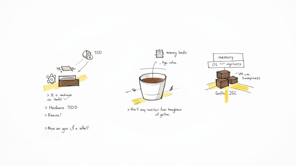
Hardware: The Bedrock of Low Latency

Honestly, the single most impactful hardware decision you can make is your storage. For Kafka's log directories, using Solid-State Drives (SSDs) instead of traditional Hard Disk Drives (HDDs) is non-negotiable for low-latency pipelines. The difference in random I/O performance is night and day, and it dramatically cuts down the time it takes to commit messages to disk.

Memory is just as important, but not just for the JVM heap. Kafka was designed to lean heavily on the operating system's page cache to serve reads without ever touching the disk. Giving your brokers plenty of RAM—we're often talking 32GB or more—lets the OS keep hot data segments cached, delivering near-instantaneous reads to your consumers.

Your hardware choices set the absolute performance ceiling for your cluster. Investing in fast SSDs and ample RAM isn't just a good idea; it's a prerequisite for consistently hitting sub-second latency. You simply can't tune your way out of slow hardware.

Operating System Tweaks for Peak Efficiency

Once the hardware is solid, you can make some targeted OS-level adjustments to squeeze out even more performance. On Linux, which is the de facto standard for Kafka, a few key settings can make a surprising difference.

One of the first things we always look at is vm.swappiness. This little parameter tells the OS how aggressively it should swap memory pages to disk. For a dedicated Kafka broker, you want to avoid swapping like the plague, as it introduces massive, unpredictable latency spikes.

• Actionable Tip: Set vm.swappiness=1 on your broker machines. This tells the kernel to only swap when it's absolutely necessary to prevent an out-of-memory error. This keeps your Kafka processes snappy and responsive.

Another critical area is the file system. You’re likely using a modern filesystem like XFS or ext4, which is great. But you also need to ensure the open file handle limit is high enough. Kafka opens a lot of file handles for its log segments, and if you hit the limit, the broker can crash. A value of 100,000 or higher is a safe starting point for most production workloads.

Taming the JVM for Predictable Performance

Finally, we get to the JVM itself. As a Java application, Kafka's performance is intrinsically tied to how the JVM manages memory—especially garbage collection (GC). A long "stop-the-world" GC pause can freeze a broker for hundreds of milliseconds, completely blowing up your sub-second SLOs.

Your goal here is simple: use a low-pause garbage collector. The G1 Garbage Collector (G1GC) is the default in modern Java versions and is a solid starting point. For workloads that demand the absolute lowest pause times, the Z Garbage Collector (ZGC) is an even better choice, often keeping pauses well below 10 milliseconds. For a deeper dive into how these system-level factors impact performance, check out our guide on how to reduce latency in data systems.

No matter which collector you pick, proper heap sizing is key. A classic mistake is giving Kafka a massive heap, thinking more is better. This can actually backfire by leading to longer GC pauses. We've found a heap size between 6-8GB is often the sweet spot, leaving the rest of the system's memory free for that crucial OS page cache. Fine-tuning the entire stack like this is the final, crucial step in building truly resilient and fast Kafka pipelines.

When Does a Managed Kafka Solution Make More Sense?

Trying to achieve sub-second pipelines by tuning Kafka yourself is a serious commitment. While having full control over a self-managed cluster is powerful, it comes with a massive operational price tag that isn't always worth paying. The endless cycle of tuning, patching, monitoring, and firefighting demands specialized expertise and drains engineering hours.

At some point, you have to ask the tough question: does our team deliver its best value by managing infrastructure, or by building the applications that run on it? If your focus is on your product, not on becoming Kafka infrastructure gurus, that's a huge sign it's time to look at a managed service.

Triggers for Offloading Kafka Management

There are a few tell-tale signs—both in your business and in your tech stack—that the scales are tipping. When the operational headache starts to outweigh the benefits of direct control, it's time to consider a change. Spotting these signs early can save you a world of pain and wasted resources.

A managed platform might be the right move if you're dealing with:

• Limited In-House Expertise: Your team is sharp, but they don't have years of battle-tested experience running Kafka in production. The learning curve is brutal, and a single mistake can be incredibly costly.
• Strict Uptime and Latency SLAs: Your business can't afford downtime or slow performance, but you don't have a dedicated 24/7 on-call team ready to jump on every issue.
• A Sky-High Total Cost of Ownership (TCO): Once you add up the salaries for dedicated engineers, the cost of emergency troubleshooting, and the opportunity cost of pulling them off feature work, a self-hosted cluster is often far more expensive than a managed service subscription.

A managed Kafka solution essentially takes the immense complexity of the entire stack off your plate. Instead of losing sleep over JVM garbage collection pauses or OS-level file handle limits, your team can focus on what they do best: building the producer and consumer logic that drives your business forward.

The True Cost of Self-Management

The monthly bill for your cloud servers is just the beginning. The real cost of running Kafka yourself is the engineering time siphoned away by tasks that don't add a single new feature to your product. This hidden cost includes everything from the initial setup and nerve-wracking upgrades to diagnosing obscure performance bottlenecks and scrambling to recover from broker failures in the middle of the night.

A managed service turns this unpredictable operational mess into a predictable monthly expense. This shift not only makes budgeting easier but also frees up your most valuable asset—your engineers—to actually innovate. Platforms that handle all that underlying complexity offer a much cleaner, faster path to high-performance pipelines without the operational drag.

To dig deeper, you can explore the benefits of using a fully managed Kafka platform in our detailed guide. It’s often the smartest way to hit your sub-second goals without burning out your team.

Ready to achieve sub-second data pipelines without the operational overhead? Streamkap provides a fully managed Kafka and Flink platform, leveraging real-time CDC to power your event-driven architecture. Let our experts handle the infrastructure while you focus on building what matters. Explore Streamkap today.